Genetic Algorithm for The Traveling Salesman Problem
This was my final project for CP407: Analysis of Algorithms during block 7 2016. I wanted to share it with you because I think it shows of the most classic problems in computer science, and demonstrates a really fascinating biologically inspired way of solving it. Before I bore you with any words, first look at the pretty animation that is the result:
So what's going on here? First let me give you some background.
The Traveling Salesman Problem (TSP) is a classic problem in Computer Science: Given a set of cities, what is the shortest way to visit each city only once before returning to the starting city? The TSP is in a set of problems called NP-Complete, which means it can easily be translated to all sorts of useful optimization problems. Some examples are aligning DNA sequences, packing things in shipping containers or files on hard drives, and matching med students with hospitals for residency.
This is a really tough problem. The most straightforward approach is to enumerate all of the possible 'tours' and pick the one with the shortest length. Unfortunately, if you have N cities, then there are N possible choices for the first city in the tour, N-1 choices for the second, N-2 for the third, and so on, which leads to N*(N-1)*(N-2)*...=N! possible tours. That means that if you had a computer that could compute the length of one tour per nanosecond, with only 20 cities it would take 77 years to find the optimum tour!
There are many algorithms that take a smarter approach than this. The best one found so far is the 1962 Held-Karp algorithm, which requires only (2^N)*(N^2) steps, instead of N!. This is much better, but it is still exponential time (because of the 2^N), which gets prohibitively slow at reasonable sizes (for 50 cities, with each step taking a nanosecond, we're back up to 89 years. Shoot dang.). In fact, it might be impossible to find an algorithm which runs in polynomial time . If you do, you'll revolutionize computer science and win a million dollars.
Genetic algorithms to the rescue!
But obviously there is some gotcha in here. Airlines plan their routes every day, DNA sequences are aligned, shipping companies aren't going broke because of poor packing, and med students aren't totally getting screwed (Right?...). The way that this is possible is that we can find an approximately optimum solution in much shorter time, and this is good enough for most real life situations.
There are many of these inexact algorithms, but the one we're going to look at is a Genetic Algorithm (GA). GA's are really cool, and are used all over the place to solve optimization problems using the power of evolution.
Here is how they work. You have a "population" of potential solutions. Some of them are more "fit" than others. In each "generation," the individuals mutate, and reproduce with each other, with the more fit individuals having a higher chance. Over time the population becomes more and more fit, eventually converging on a close to optimal solution, just like populations of organisms do in nature!
For the TSP, each individual is simply a tour through all the cities. The other aspects of the algorithm aren't so clear. For instance, what does it mean to 'mutate' a tour? Maybe you just swap two cities in your itinerary, so instead of going A-B-C-D-E-F-G, you randomly choose C and F, and the tour mutates to A-B-F-D-E-C-G. Maybe you chop the tour into chunks and reorder them, so that A-B-C-D-E-F-G is split into A-B, C-D-E, and F-G, and reordered to A-B-F-G-C-D-E.
What is 'fitness' and how do we choose the more fit parents? It would make sense for this to somehow be related to the length of the tour. Maybe we just skim off the top 10 individuals from the population? How about selecting the parents with a lottery, weighting their chances by their tour lengths? Should we use the actual length of the tour, so that a tour with half the length is twice as likely to be picked as some other tour? Or perhaps it makes sense to not care about the actual lengths of the tours, and instead focus on how the tours rank compared to each other.
As you can see, there are many ways to tailor a genetic algorithm for a problem, and the choices you make have a huge impact on the performance.
My implementation
Here is how I decided to implement the GA. I gained inspiration from an article called . "An Evolutionary Approach for the TSP and the TSP with Backhauls." by Süral et al, but had to tweak and expand his outline, because it was still fairly general. You can find my project folder in a GitHub repository here, follow along with this if you like.
I wanted to test the algorithm on standard, real-life problems, and I wanted to be able to compare the results of the GA to the real, optimal tour. Therefore, I used a standard library of TSP problems called TSPLIB, that offered many sample instances of various types, many with verified solutions. To make the job easier on myself, I only used problems that represented cities as points in two dimensions. Thus, I could plot the cities and tours easily, to double check my work, and to make a more intuitive demonstration. This also made it so that the problem was symmetrical, which means the distance from A to B is the same as from B to A. Some instances aren't, for example when planning an airline route, flying from Anchorage to Seattle is easier than the other way because of the jet stream. Also, choosing these problems made it so that the problem is complete, meaning it is possible to get from any city to any other city.
After I defined the specifications of the problem, I had to make some choices about my algorithm. I made it so that there are 100 individuals in the population, and I just hardcoded it so that the simulation runs for 50 generations.
To choose the parents for the next generation, I used a binary selection tournament. This works by randomly selecting two individuals from the population, and the one with the shorter tour length is included in the parent pool. The two candidates are replaced, and two more randomly chosen. This repeats until the desired number of parents are picked, which in my case I set to be half of the total in the population.
To breed two individuals, first make the union of their two tours, and then perform something called the greedy nearest neighbor algorithm on this union graph to determine a reasonable child of the two parents. First, randomly choose a starting city in the union graph, greedily go to the closest city that we haven't visited yet, and repeat. Sometimes this results in dead ends, or you finish the tour prematurely, so you can pick roads and cities that aren't in the union if you paint yourself into a corner.
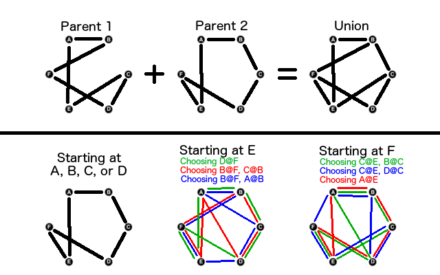
Breeding two parents to get a union graph, and then performing a greedy nearest neighbors algorithm. We assume that the cities are arranged around a hexagon. This means that B and F are equally close to A, C and E are a little bit further, and D is the furthest. Extend this preference of neighbors for the other 6 orientations. Notice the different results that you can get by starting at different cities, and by the random choices that you can make when two cities are equidistant. In some of these scenarios, you end up painting yourself into a corner and have to choose edges that aren't in the union graph so that the circuit remains legal.
To mutate an individual, you reverse a random section of the tour. For instance, with a tour A-B-C-D-E-F-G, you might randomly choose the cities C and F, and the tour becomes A-B-F-E-D-C-G. You don't want to mutate every individual every time though, or the benefits of selective breeding begin to be overshadowed by the random noise of mutation. I made it so that 5% of the population is mutated in every generation.
There are a few more details to explain. If an individual isn't picked in the parent selection tournament, that individual's 'genes' aren't passed on to the next generation. That means that if we are unlucky we could accidentally throw out the fittest individual from the previous generation! To prevent this, I made it so the top 5% of the population is guaranteed to persist between generations.
There are a few more details to explain. If an individual isn't picked in the parent selection tournament, that individual's 'genes' aren't passed on to the next generation. That means that if we are unlucky we could accidentally throw out the fittest individual from the previous generation! To prevent this, I made it so the top 5% of the population is guaranteed to persist between generations.
Results
Take a look at the algorithm working on some other instances of the TSP:
|
|
|
|
|
|
As you can see, the performance is ok. It often finds sequences of cities that are perfect, but then makes really large, really stupid looking jumps! A human could probably even do better. I think the long jumps are the result of the greedy algorithm during the breeding of the two parents. The algorithm keeps on adding the next closest city, but then "paints itself into a corner" and is stuck with making a large jump. Depending on the instance, the best solution found by the GA varies between about 1% and 16% worse than the real solution. It is interesting to note that the larger the problem, and the more cities there are, the worse the performance is.
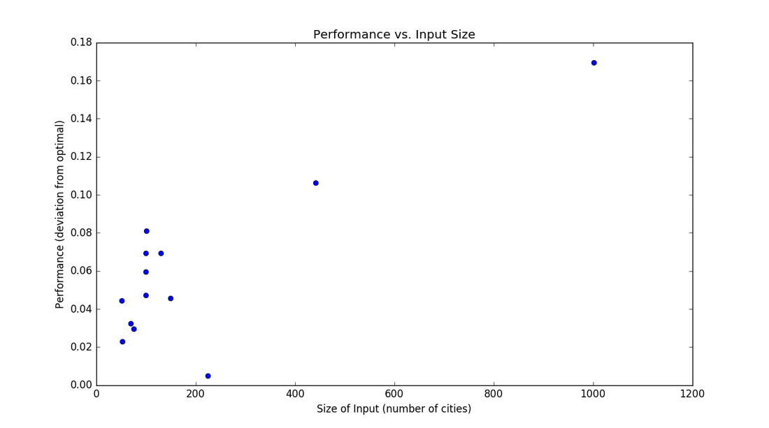
Even though this algorithm isn't incredibly accurate, it sure is fast. The huge instances of more than 2000 cities took less than 15 seconds to run on my computer! That's because instead of requiring N! or 2^N*N^2 steps, this is close to linear time N. This is a bit more complicated to find, but read the Complexity section below to learn more.
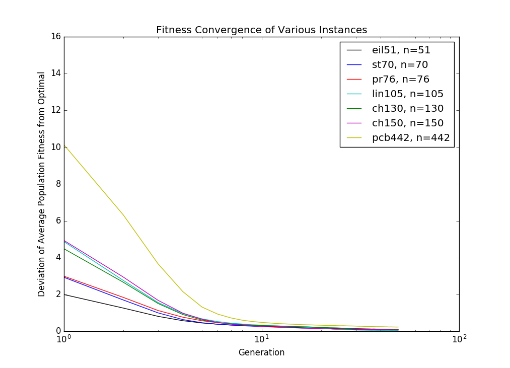
It also is interesting to look at how the population converges. At some point in the simulation, one solution takes over the gene pool, and drives all the other individuals to extinction. Then, improvements in the solution only come from mutations in individuals, not from crossover from parents, the quality of the solutions levels off, and you might as well call it good. For this algorithm, this seems to happen at around generation 15, regardless of the size of the input.
It also is interesting to look at how the population converges. At some point in the simulation, one solution takes over the gene pool, and drives all the other individuals to extinction. Then, improvements in the solution only come from mutations in individuals, not from crossover from parents, the quality of the solutions levels off, and you might as well call it good. For this algorithm, this seems to happen at around generation 15, regardless of the size of the input.
Complexity
One of the main reasons to use a Genetic Algorithm is to avoid the huge cost of searching the entire solution space with a branch and bound or some other deterministic algorithm. So what is the time complexity of this genetic algorithm?
Let's define some of the input sizes to this algorithm. Perhaps the one we care about most is n, the number of cities in the instance. However, we also need to think about the population size p and the number of generations g that we simulate for, since these two things have a huge impact on the quality of a solution.
Each iteration, there are a few things that need to happen. First, we have to find the k fittest individuals that will persist to the next generation. This partial sorting is of order p + k*lg(k), and since at most we could preserve the entire population, this step is order p*lg(p). The next step is to select parents for the next generation. With the binary tournament selection, sampling and choosing the fittest individual is constant. Since at most we can select p parents for the next generation, this step is order p. Next, we perform the Nearest Neighbor Algorithm to breed children for the next generation. Here, we must first construct a union graph of both paths, which has a cost of 2n, since each path has n edges. Then we must perform the greedy search on this graph, which will take n steps to complete. Within each step, since the simple union graph might not yield a legal solution, we may have to check through all of the n cities in the complete graph before we find one that we haven't visited. Also, we need to evaluate this new child, which takes n steps to add up all the edges. This means that the cost for completing the NNA, and of breeding one child is of order n^2, the cost for breeding the entire population is order p*n^2. The last step is to mutate the population, which might take n*p time if we mutate the entire chromosome of every individual in the population.
Since the costliest operation in each iteration, breeding, is order p*n^2, and we go through this loop g times, the order of the entire algorithm is g*p*n^2. Our observations on the convergence for different values of n support the idea that it is possible to hold g constant as n increases. Also, the research community has found that there is limited benefit for increasing population size with increasing n. Assuming that we can hold g and p constant, this algorithm is only order n^2. Actually, since over the course of the simulation the population stabilizes so that each city is connected to one of its very close neighbors, the lookup time for the next nearest city in the greedy nearest neighbor algorithm approaches constant time. This means that the complexity is much closer to n, linear time! Either way, this is a drastic improvement on the dynamic programming complexity of n^2*2^n.
